Substitutional Point Defects in Graphene (Formation Energy and Band Structure)

1. Introduction

This tutorial calculates the formation energy and the electronic band structure of the trimerized pyridine-type C₂₈N₃ defect in graphene, reproducing results from the following manuscript:

Manuscript

Yoshitaka Fujimoto and Susumu Saito, "Formation, stabilities, and electronic properties of nitrogen defects in graphene", Physical Review B, 2011. DOI: 10.1103/PhysRevB.84.245446. ¹

This tutorial builds upon the Substitutional Point Defects in Graphene tutorial, where the pristine 4×4 graphene cell and the C₂₈N₃ defect are created. Both properties are calculated with Quantum ESPRESSO on the same cell.

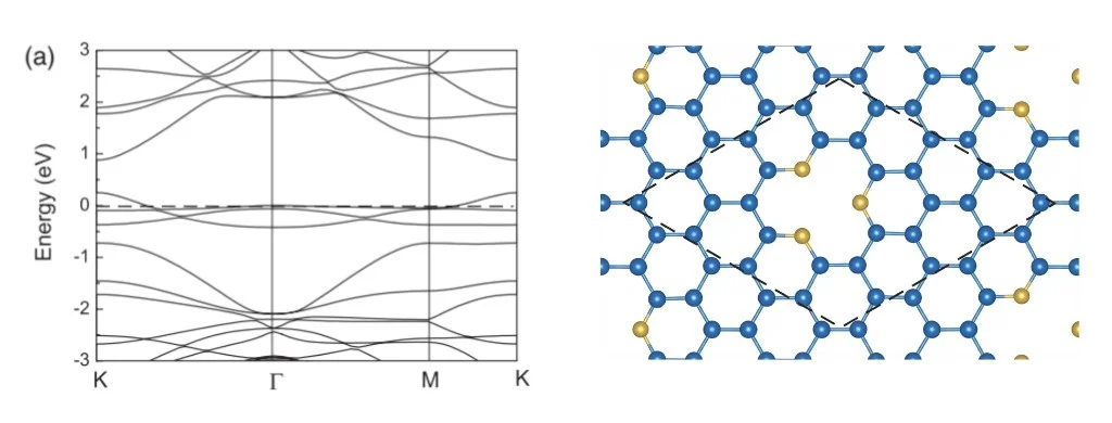
The figure below shows the band structure and atomic structure of N-doped graphene from the manuscript (Figure 3a):

The calculation uses Density Functional Theory (DFT) with the Local Density Approximation (LDA), following the method described in the manuscript. Section 4 lists the settings and the single deviation from it.

2. Prerequisites

The notebook loads two materials from the uploads folder by exact name and raises when either is missing: graphene 4x4, the pristine reference cell that supplies the carbon chemical potential, and graphene 4x4 N3V pyridinic (C28N3), the defective cell. Both are created and saved by the Substitutional Point Defects in Graphene tutorial, which should be run first. The nitrogen reference is resolved from Standata and needs no upload.

3. Workflow overview

The formation energy is assembled in the notebook from three total energy jobs, as defined in Section II of the manuscript:

E_f = E(C₂₈N₃) − 28 μ_C − 3 μ_N

where μ_C is the total energy of the pristine 4×4 cell per atom and μ_N that of the nitrogen reference cell per atom. A fourth job calculates the band structure of the same defective cell. The steps are:

1. Set up the environment and parameters: material names, DFT model, relaxation switch, and compute settings
2. Authenticate and initialize API client: connect to the platform
3. Load the materials: the pristine and defective cells from the uploads folder, the nitrogen reference from Standata
4. Configure the shared model and k-grid: one DFT model and a per-material k-grid for every job below
5. Configure compute resources: select cluster, queue, and processor settings
6. Relax the defective cell: only when RELAX is set, reusing a relaxed structure already saved on the account
7. Run the Total Energy jobs: the defective, pristine, and nitrogen cells
8. Run the Band Structure job: on the defective cell
9. Retrieve the results: the band structure plot, the formation energy, and the comparison with Table I

4. Calculation parameters

4.1. Relaxation switch

One switch in cell 1.3 decides which geometry both properties are calculated on:

# NOTE: set to True for results close to the manuscript (relaxes C28N3 once, ~1 h); the formation
# energy and the band structure both depend on it.
RELAX = False

The relaxation keeps the cell fixed, is spin-polarized, and converges to the manuscript's 0.05 eV/Å (RELAXATION_SETTINGS in cell 1.4). It runs on the defective cell only: the pristine cell is at its minimum already.

4.2. DFT model parameters

Cell 1.4 sets the model shared by every job:

# NOTE: the manuscript's value needs its own settings — Troullier-Martins norm-conserving LDA;
# its 4x4 cell, 50 Ry cutoff and 6x6x1 k-grid are matched below, its pseudopotentials are not.
MODEL_SUBTYPE = "lda"
FUNCTIONAL = "pz"
PSEUDOPOTENTIAL_TYPE = "us"  # GBRV ultrasoft, the only LDA family the platform publishes for C and N
ECUTWFC = 50   # Ry, Fujimoto & Saito Sec. II
ECUTRHO = 200  # Ry, GBRV's recommended charge-density cutoff

KPOINT_DENSITY = 7  # points per Å⁻¹; gives 6 x 6 x 1 on the 4x4 cell, Fujimoto & Saito Sec. II
MODEL_TAG = f"{FUNCTIONAL}-{PSEUDOPOTENTIAL_TYPE} {ECUTWFC}-{ECUTRHO}Ry k{KPOINT_DENSITY}"

SCF_UNIT = "pw_scf"
BANDS_UNIT = "pw_bands"
RELAX_UNIT = "pw_relax"
# C28N3 carries 127 valence electrons, so its ground state is a doublet.
SPIN_SETTINGS = {
    DEFECTIVE_NAME: {"nspin": 2, "tot_magnetization": 1},
    PRISTINE_NAME: {"nspin": 1},
    NITROGEN_NAME: {"nspin": 1},
}
RELAXATION_SETTINGS = {"forc_conv_thr": 1.9e-3, "nstep": 100}  # 0.05 eV/Å, Fujimoto & Saito Sec. II
# Names the relaxation job; the relaxed structure itself is found by content hash.
RELAX_TAG = f"{MODEL_TAG} f{RELAXATION_SETTINGS['forc_conv_thr']}"

KPATH_STEPS = 20
KPATH = [
    {"point": "K", "steps": KPATH_STEPS},
    {"point": "Γ", "steps": KPATH_STEPS},
    {"point": "M", "steps": KPATH_STEPS},
    {"point": "K", "steps": 1},
]

The functional, the 4×4 cell, the 50 Ry cutoff, and the 6×6×1 k-grid are the manuscript's own. The pseudopotentials are not: the platform publishes no norm-conserving LDA set for carbon or nitrogen — the nc family is published under PBE only — so the GBRV ultrasoft set is the only settable LDA choice, and it stands in for the manuscript's Troullier-Martins norm-conserving set. ECUTRHO = 200 Ry is the density cutoff recommended for that set.

The nitrogen chemical potential is taken from Standata's solid nitrogen (mp-154), where the manuscript uses the free N₂ molecule; the platform carries no free molecule. Both offsets are named again in the notebook's comparison output.

5. Step-by-step instructions

5.1. Open the notebook

Navigate to the API examples repository and open the simulation notebook:

other/materials_designer/specific_examples/defect_point_substitution_graphene_SIMULATION.ipynb

5.2. Set the material names

Cell 1.2 names the materials the notebook loads:

# Names saved by defect_point_substitution_graphene.ipynb.
PRISTINE_NAME = "graphene 4x4"
DEFECTIVE_NAME = "graphene 4x4 N3V pyridinic (C28N3)"
# Standata's solid nitrogen -- the platform carries no free N2 molecule.
NITROGEN_NAME = "N2, Nitrogen, FCC (P2_13) 3D (Bulk), mp-154"

5.3. Run the notebook

Execute all cells by selecting Run > Run All Cells.

The notebook will:

1. Authenticate with the platform and initialize the API client
2. Load the two graphene cells and the nitrogen reference, and save all three to the platform
3. Relax the defective cell, when RELAX is set
4. Submit one Total Energy job for each cell that does not have one yet
5. Submit the Band Structure job on the defective cell
6. Display the band structure, the formation energy, and the comparison with the manuscript

5.4. Monitor progress

Each set of jobs is polled every 60 seconds and the notebook waits for it to finish before moving on. The Total Energy jobs and the band structure job take minutes; the optional relaxation takes about an hour.

5.5. Read the results

Section 9 of the notebook plots the band structure along the K → Γ → M → K path and prints the formation energy beside the manuscript's value, under the regime it was calculated in — relaxed defect or unrelaxed SCF.

6. Expected results

The formation energy is compared with Table I of the manuscript, within a tolerance of 15 % of the published value:

Quantity	Manuscript	This tutorial, RELAX = True
Formation energy of C₂₈N₃	2.51 eV (Table I)	TODO(live run)
Total magnetic moment	0.89 μB (Sec. III C)	TODO(live run)

Two known offsets are covered by that tolerance: the nitrogen chemical potential comes from solid N₂ rather than the free molecule, and the GBRV ultrasoft set stands in for the norm-conserving one. The default RELAX = False run calculates both properties on the unrelaxed geometry and is not expected to match the manuscript.

6.1. Read the magnetic moment

The magnetic moment is a manual check: the platform exposes no magnetization property and the notebook does not parse job files. Open the C₂₈N₃ Total Energy job on the platform, select its Files tab, and read the total magnetization line of pw_scf.out.

6.2. Comparison with published results

The figure below compares the band structure from the Fujimoto & Saito manuscript (left) with the calculated results (right):

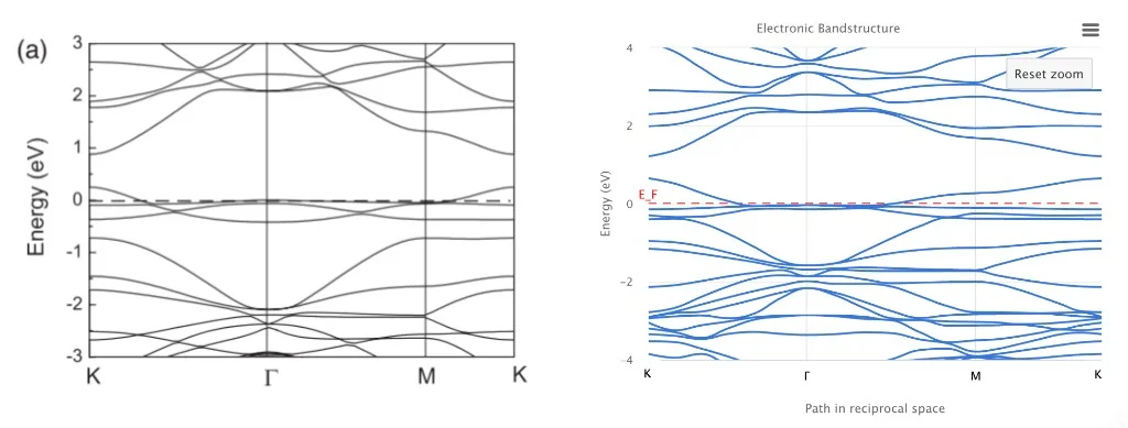
The check is for the three acceptor-like states near the Fermi level reported in Section III C, along the K → Γ → M → K path.

7. Customization options

7.1. Modify the K-path

The path is the KPATH list in cell 1.4. Add or replace high-symmetry points there, or raise KPATH_STEPS for a denser sampling between them. Γ is the Greek capital gamma (U+0393); the visually identical Cyrillic Г is not resolved as a point of the reciprocal lattice.

7.2. Adjust computational resources

Modify the compute parameters in cell 1.3:

CLUSTER_NAME = "001"  # specify full or partial name i.e. "cluster-001" to select
QUEUE_NAME = QueueName.OR
PPN = 16  # queue OR on cluster-001 allows at most 16 cores per node
TIME_LIMIT = "12:00:00"  # covers the optional relaxation (~1 h)

7.3. Run the relaxed regime

Set RELAX = True in cell 1.3 to reproduce the manuscript. The notebook then relaxes the defective cell before submitting anything else, takes both properties from the final structure of that job, and saves it as graphene 4x4 N3V pyridinic (C28N3) relaxed. A later run finds that structure on the account and skips the relaxation.

8. Troubleshooting

8.1. Material not found

Loading raises when either name is missing from the uploads folder. Earlier versions of the structure notebook saved one material, named N-doped Graphene; an uploads folder left from one of those does not satisfy this notebook. Re-run the structure creation tutorial, which saves both materials under the names in cell 1.2.

8.2. Cluster not found

Section 5 raises ValueError: Cluster '001' not found and lists the available hostnames when the account has no cluster matching CLUSTER_NAME. Set CLUSTER_NAME to one of the listed hostnames, or to None to take the first available cluster.

8.3. The default run does not reproduce the manuscript

With RELAX = False the comparison block ends with Reproduces Fujimoto & Saito (2011): no (unrelaxed SCF). Both published quantities belong to the relaxed geometry, so reproducing them takes the relaxed regime of Section 7.3.

9. Interactive JupyterLite notebook

The following JupyterLite notebook calculates the formation energy and the band structure of the C₂₈N₃ defect in graphene. Select Run > Run All Cells.

⛶ Full Screen

10. References

---

1. Yoshitaka Fujimoto and Susumu Saito. Formation, stabilities, and electronic properties of nitrogen defects in graphene. Phys. Rev. B, 84:245446, Dec 2011. URL: https://link.aps.org/doi/10.1103/PhysRevB.84.245446. ↩